Solving KdV Solitons with Upwinding Operators

The KdV equation is of the form uₜ + αuuₓ + βuₓₓₓ = 0. Here we'll use α = 6, β = 1 for simplicity of the true solution expression.

1-Soliton solution using Upwind Difference

The analytical expression for the single soliton case takes the form u(x,t) = (c/2)/cosh²(√c * ξ/2).

c > 0 (wave speed) ; ξ = x - c*t (moving coordinate)

using Test
using DiffEqOperators, OrdinaryDiffEq, LinearAlgebra

# Space domain and grids
N = 21
Δx = 1/(N-1)
c = 1
x = -10:Δx:10;

# solution of the single forward moving wave
ϕ(x,t) = (1/2)*sech.((x .- t)/2).^2 

# Discretizing the PDE at t = 0
u0 = ϕ(x,0);
du = zeros(size(x)); 

# Declaring the Upwind operator with winding = -1 since the wave travels from left to right 
A = UpwindDifference{Float64}(1,3,Δx,length(x),-1);

# Defining the ODE problem
function KdV(du, u, p, t)
	bc = GeneralBC([0,1,-6*ϕ(-10,t),0,-1],[0,1,-6*ϕ(10,t),0,-1],Δx,3) 
	mul!(du,A,bc*u)
end

single_solition = ODEProblem(KdV, u0, (0.,5.));

# Solving the ODE problem 
soln = solve(single_solition,Tsit5(),abstol=1e-6,reltol=1e-6);

# Plotting the results, comparing Analytical and Numerical solutions 
using Plots
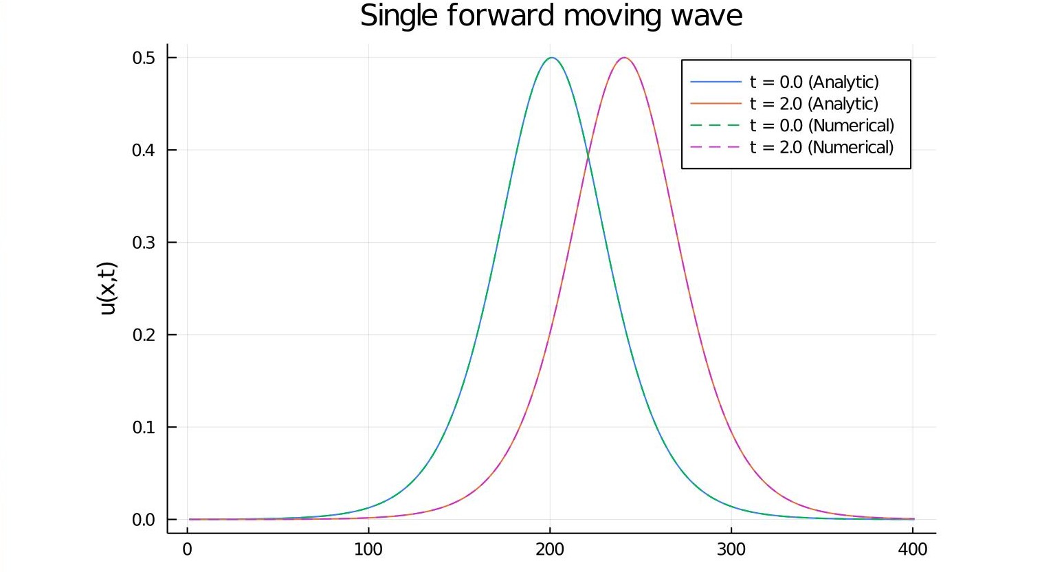
plot(ϕ(x,0), title  = "Single forward moving wave", yaxis="u(x,t)", label = "t = 0.0 (Analytic)")
plot!(ϕ(x,2), label = "t = 2.0 (Analytic)")
plot!(soln(0.0), label = "t = 0.0 (Numerical)",ls = :dash)
plot!(soln(2.0), label = "t = 2.0 (Numerical)",ls = :dash)